Color Image into Grayscale using Python Image Processing Libraries | An Exploration

Processing Libraries used:

Libraries for image data wrangling:

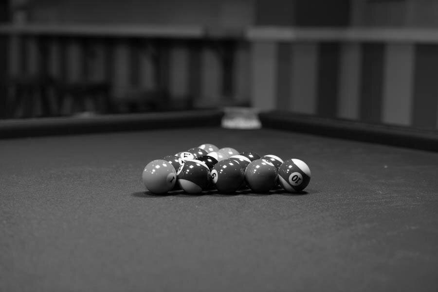
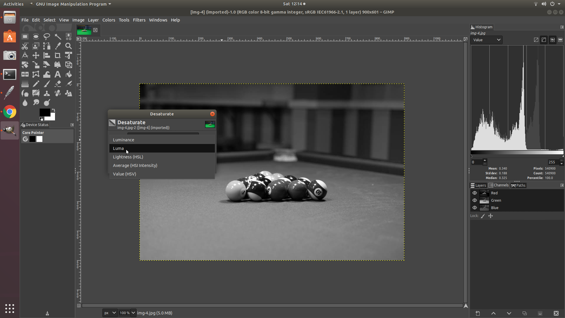
To get started, lets access the image file and bring it inside our script. Let us use the python os module to access and read the file into the script

We will also be importing "Image" module from Pillow(PIL) library

 1
 2
 3
 4
 5
 6
 7
 8
 9
10
11
12
13
14
15
16'''Exploring grayscale with Python using PIL, Skimage, NumPy and Matplotlib Libraries'''

import os
from PIL import Image, ImageColor, ImageOps
from skimage import color
import numpy as np
import matplotlib.pyplot as plt
import matplotlib.style as style
import matplotlib.image as mpimg
from exception import IOError

'''Opening an image using Python's os module'''

path = os.path.join(os.path.expanduser('~'), 'Desktop','color','img-4.jpg')
img = Image.open(path)
img.show()

Lets read the image properties using PIL.image functions. To check if the right image is read, let's open it in the default image previewer of your OS.

 1
 2
 3
 4
 5
 6
 7
 8
 9
10
11img = Image.open(path)
img.show() #preview the image in the default image editor of your OS

'''Image Properties'''
print("filename:",img.filename)
print("format:", img.format)
print("mode:", img.mode)
print("size:", img.size)
print("width*height", img.width, "*", img.height)
print("palette:", img.palette)
print("Image Info:", img.info)

The image properties

filename: /home/pk/Desktop/color/img-4.jpg

format: JPEG * mode: RGB

size: (900, 601)

width*height: 900 * 601

palette: None

imgInfo: dict_keys(['exif', 'dpi', 'photoshop', 'adobe', 'adobe_transform', 'icc_profile'])

Converting to Grayscale

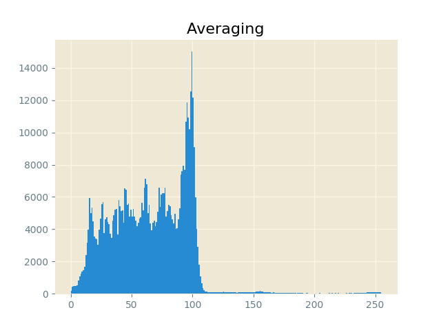
Method 1: Averaging the R,G,B values.(non-linear)

This is the most basic of all grayscale conversion method. We take the average of R,G,B values of each pixel to arrive at a single value(ranging from 0 (black) to 255 (white).

As quoted here :

Some computer systems have computed brightness using (R+G+B)/3. This is at odds with the properties of human vision

Method 1: Averaging - R,G,B values 

Y = (R+G+B)/3

1
2
3
4
5
6
7
8
9"""Method 1 - Averaging - R,G,B values """ 

#Python's Lambda(anonymous) expression. Apply simple math and convert to a list(of pixles)

AllPixels = list(map(lambda x: int((x[0] + x[1] + x[2])/3), list(img.getdata()))) 
GreyscaleImg1 = Image.new("L", (img.size[0], img.size[1]), 255)   #instantiate an image
GreyscaleImg1.putdata(AllPixels)   #Copies pixel list to this image
GreyscaleImg1.show()               #preview image
plotHist(GreyscaleImg1,"Averaging")  #plot a histogram

The human eye always interprets different colors in a different way. The weights ranging in the order of Green, Red and Blue.

Taking into consideration the color perception, we have methods 2 and 3 below.

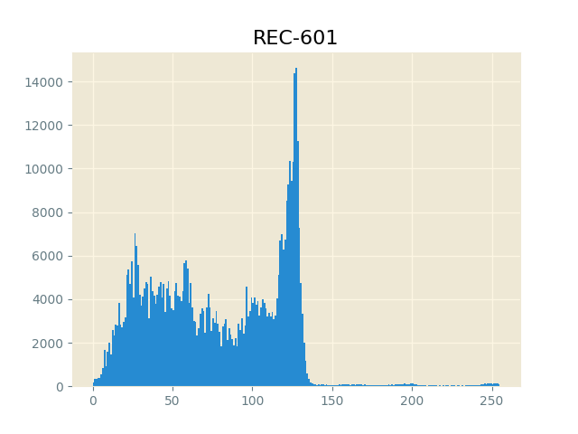
Method 2: LUMA-REC-601(non-linear)

Again quoting Charles Poynton,

If three sources appear red, green and blue, and have the same radiance in the visible spectrum, then the green will appear the brightest of the three because the luminous efficiency function peaks in the green region of the spectrum. The red will appear less bright, and the blue will be the darkest of the three. As a consequence of the luminous efficiency function, all saturated blue colors are quite dark and all saturated yellows are quite light. If luminance is computed from red, green and blue, the coefficients will be a function of the particular red, green and blue spectral weighting functions employed, but the green coefficient will be quite large, the red will have an intermediate value, and the blue coefficient will be the smallest of the three.

Method 2 - LUMA-REC-601

Y = ( R * 299/1000 + G * 587/1000 + B * 114/1000 )

1
2
3
4
5
6
7
8
9""""""Method 2 - LUMA-REC-601"""  """ 

#Python's Lambda(anonymous) expression. Apply simple math and convert to a list(of pixles)

AllPixels = list(map(lambda x: int(x[0]*(299/1000) + x[1]*(587/1000) + x[2]*(114/1000)), list(img.getdata())))
GreyscaleImg2 = Image.new("L", (img.size[0], img.size[1]), 255)   #instantiate an image
GreyscaleImg2.putdata(AllPixels)   #Copies pixel list to this image
GreyscaleImg2.show()               #preview image
plotHist(GreyscaleImg2,"REC-601")  #plot a histogram

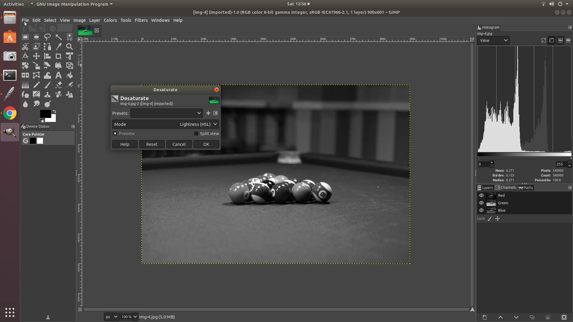
The PIL image module has a convert function that helps to convert an image from one mode to another. To convert to grayscale, pass in "L" (luminance) as a mode parameter. When translating a color image to black and white (mode “L”), the library uses the ITU-R 601-2 luma transform

1
2
3
4#When translating a color image to black and white (mode “L”), the library uses the ITU-R 601-2 luma transform:

grayImg = img.convert('L')
grayImg.show()

Learn more about LUMA REC.601 here.

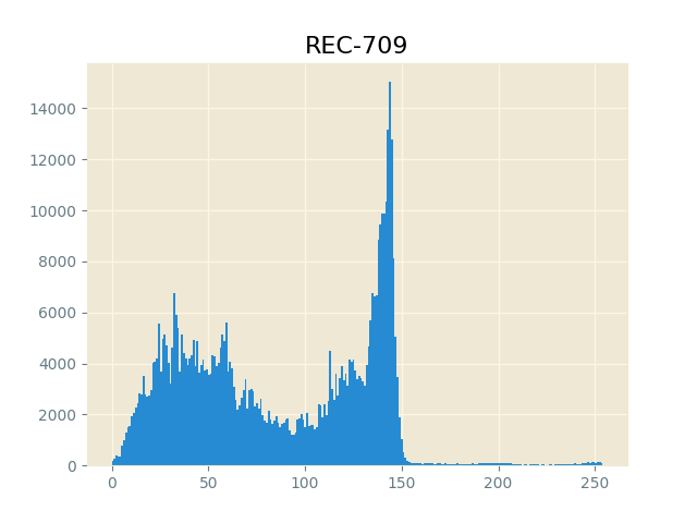
Method 3 - LUMA-REC.709(non-linear)

Both REC.601 and REC.709 considers the difference in color perception( and hence different coefficients for R,G, B). But the major difference is as follows:

Quoting Charles Poynton, with respect to REC.60:

The coefficients 0.299, 0.587 and 0.114 properly computed luminance for monitors having phosphors that were contemporary at the introduction of NTSC television in 1953. However, these coefficients do not accurately compute luminance for contemporary monitors

Where as REC.709:

Contemporary CRT phosphors are standardized in Rec. 709 [9], to be described in section 17. The weights to compute true CIE luminance from linear red, green and blue (indicated without prime symbols), for the Rec. 709, are these:

Method 2 - LUMA-REC.709

Y = 0.2125 * R + 0.7154 * G + 0.0721 * B

1
2
3
4
5
6
7
8
9""""""Method 3 - LUMA-REC-709"""  """ 

#Python's Lambda(anonymous) expression. Apply simple math and convert to a list(of pixles)

AllPixels = list(map(lambda x: int(x[0]*(212/1000) + x[1]*(715/1000) + x[2]*(72/1000)), list(img.getdata())))
GreyscaleImg3 = Image.new("L", (img.size[0], img.size[1]), 255)   #instantiate an image
GreyscaleImg3.putdata(AllPixels)   #Copies pixel list to this image
GreyscaleImg3.show()               #preview image
plotHist(GreyscaleImg3,"REC-709")  #plot a histogram

Let’s dig down to see, how the math works at the pixel level:

The results from the grayscale conversion methods:

Averaging the R,G,B values

Y = (R+G+B)/3

REC-601

Y = ( R * 299/1000 + G * 587/1000 + B * 114/1000 )

REC-709

Y = 0.2125 * R + 0.7154 * G + 0.0721 * B

GIMP-LUMA-REC-709

Y = 0.2125 * R + 0.7154 * G + 0.0721 * B

GIMP HSL

Y = (R+G+B)/3

GIMP LUMA

REC.709 (non-linearized)

 1
 2
 3
 4
 5
 6
 7
 8
 9
10
11
12
13
14
15
16
17
18
19
20
21
22
23
24
25
26def plotHist(grayImg, title):
   ImagingCore= grayImg.getdata()
   print(ImagingCore)  #<ImagingCore object at 0x7f952e28aa10>
   print(type(ImagingCore))   #<class 'ImagingCore'>
   print(grayImg.getextrema())    #(0, 255)
   
   #Follwing returns a flat list of pixel values(ranging from 0-255). We'll convert these values into an array down below
   GrayPixels=list(grayImg.getdata()) 
   print(type(GrayPixels))    #<class 'list'>
   
   # convert the list into an array. Matplotlib accepts array as a parameter to plot histogram
   GrayPixelsArray = np.array(GrayPixels) 
   
   print (GrayPixelsArray.size) #540900 i.e width*height: 900 * 601
   print (GrayPixelsArray.shape) #(540900,)
   print (GrayPixelsArray.dtype) #int64
   print (GrayPixelsArray.ndim) #1-D array
   print(np.mean(GrayPixelsArray), 
         np.median(GrayPixelsArray),
         np.std(GrayPixelsArray),
         np.max(GrayPixelsArray), 
         np.min(GrayPixelsArray))    #64.90450730264374 66.0 31.959808127905852 255 0
   plt.style.use('Solarize_Light2')      
   plt.hist(GrayPixelsArray, bins = 255)
   plt.title(title) 
   plt.show()

Image Statistics:
+------------+---------+---------+--------+------+-----+
| Grayscale  |  Mean   | Median  |  Std   | Max  | Min |
+------------+---------+---------+--------+------+-----+
+------------+---------+---------+--------+------+-----+
| Averaging  | 64.90   |  66.0   | 31.95  | 255  |  0  |
+------------+---------+---------+--------+------+-----+
|  REC-601   | 77.76   |  76.0   | 41.38  | 255  |  0  |
+------------+---------+---------+--------+------+-----+
|  REC-709   | 86.23   |  82.0   | 47.94  | 254  |  0  |
+------------+---------+---------+--------+------+-----+

Grayscale conversion using Scikit-image processing library

We will process the images using NumPy. NumPy is fast and easy while working with multi-dimensional arrays.

For instance an RGB image of dimensions M X N with their R,G,B channels are represented as a 3-D array(M,N,3). Similarly a grayscale image is represented as 2-D array(M,N). NumPy is fast and easy when it comes to doing calculations on big arrays(large images).

We’ll use plotting functions from Matplotlib to plot and view the processed image.

To convert to grayscale(non-linear):

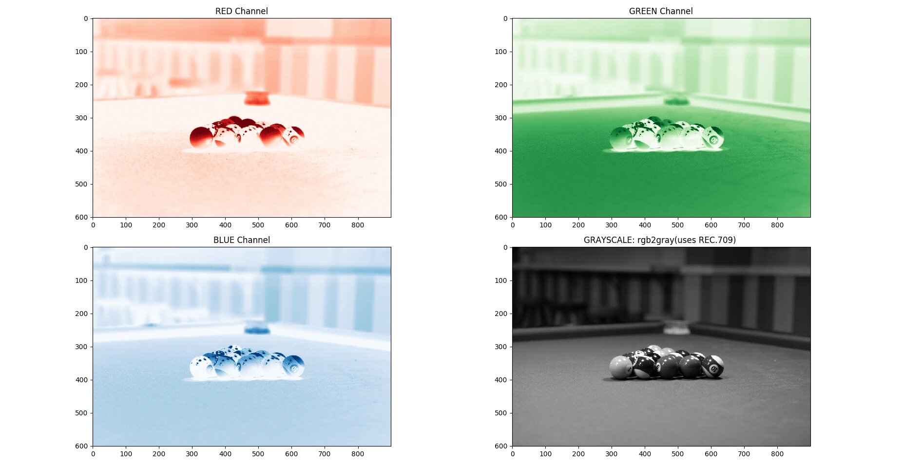
We’ll be using the inbuilt rgb2gray from the color module. rgb2gray uses REC.709. for the conversion
We’ll also manually do the REC.709 conversion calculation by working on the numpy.ndarray objects

 1
 2
 3
 4
 5
 6
 7
 8
 9
10
11
12
13
14
15
16
17
18
19
20
21
22
23
24
25
26
27
28
29
30
31
32
33
34
35
36
37
38
39
40
41
42
43
44import os
import numpy as np
import matplotlib.pyplot as plt
import matplotlib.image as mpimg
from skimage import color, io, data
from skimage.viewer import ImageViewer
from PyQt5 import QtCore, QtGui, QtWidgets

img = io.imread('/home/pk/Desktop/color/img-4.jpg')  #Fetch the image into the script

"""Reading the properties of the image"""

#plt.imshow(img)
#plt.show()
#print(img)    #Prints RGB values of each pixel across W*H as a 3D matrix(M,N,3)
#print(type(img))    #<class 'numpy.ndarray'>
#print(img.shape)    #(601, 900, 3)


"""Splitting the image into R,G,B Channels"""

R = img[:, :, 0]
G = img[:, :, 1]
B = img[:, :, 2]
Gray = color.rgb2gray(img) # REC.709 | Y = 0.2125 R + 0.7154 G + 0.0721 B 
#Gray = (R*0.212)+(G*0.715)+(B*0.072) # or do the conversion math across 3 channels

## we shall use matplotlib to display the channels

fig, ((ax1, ax2), (ax3,ax4)) = plt.subplots(nrows=2, ncols=2, figsize=(20,10))

ax1.imshow(R,cmap=plt.cm.Reds)
ax1.set_title("RED Channel")

ax2.imshow(G,cmap=plt.cm.Greens)
ax2.set_title("GREEN Channel")

ax3.imshow(B,cmap=plt.cm.Blues)
ax3.set_title("BLUE Channel")

ax4.imshow(Gray, cmap="gray")
ax4.set_title("GRAYSCALE: rgb2gray(uses REC.709) ")

plt.show()

RGB image numpy.ndarray representation. — RGB image ***numpy.ndarray*** representation.

Plot of red, green, blue, and gray conversions.

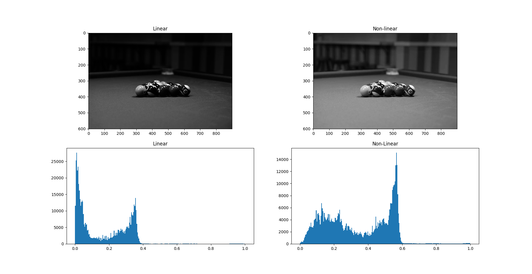
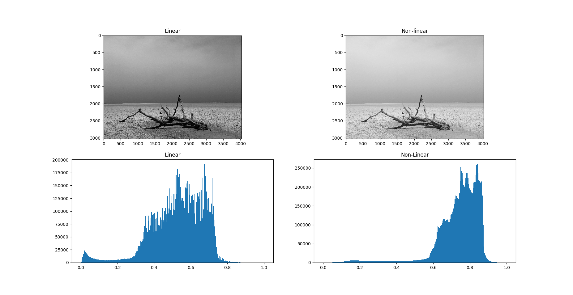
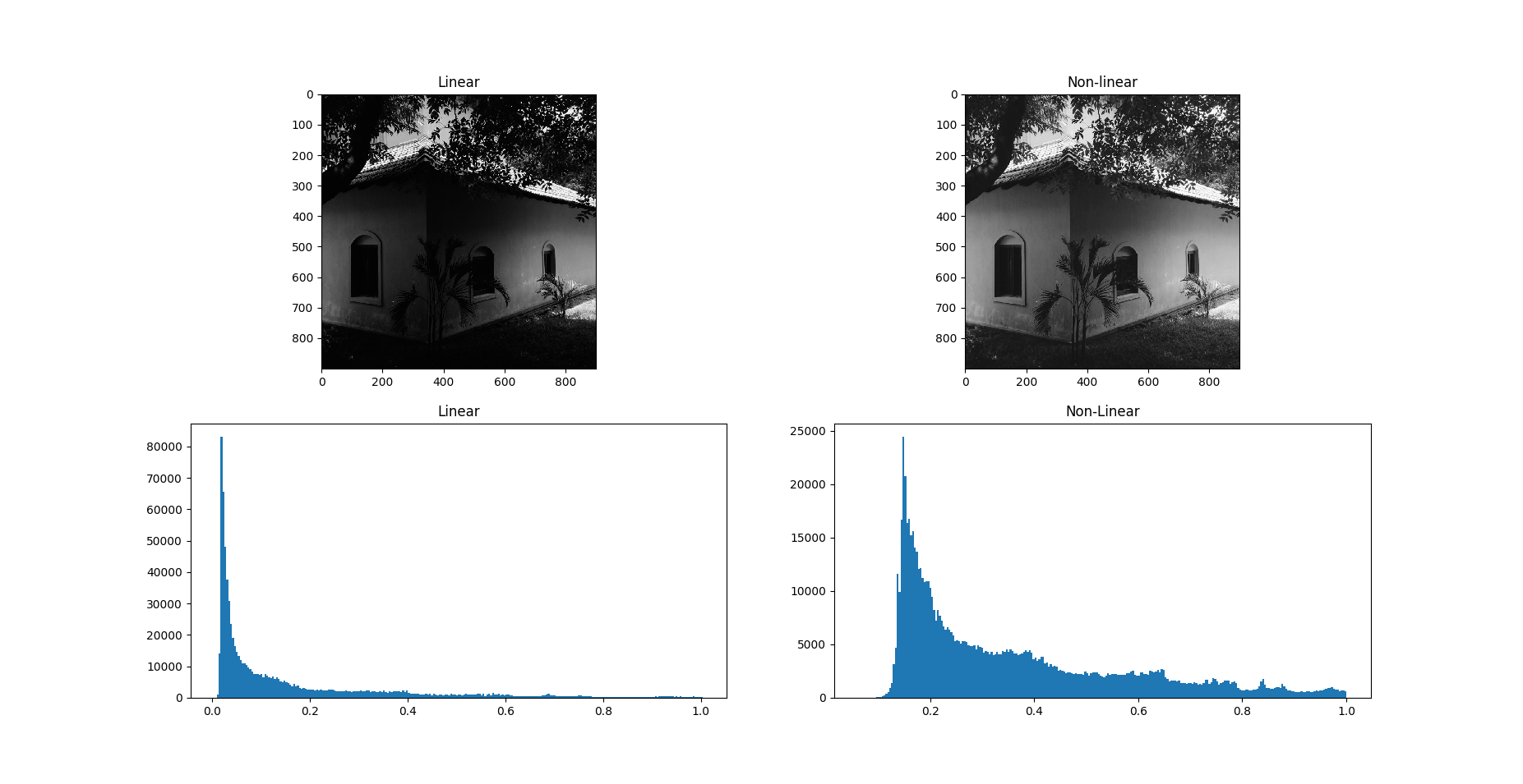
Converting to GrayScale: The right way by linearization of sRGB by applying inverse gamma function.

All RGB images are gamma encoded.

Gamma encoding of images is used to optimize the usage of bits when encoding an image, or bandwidth used to transport an image, by taking advantage of the non-linear manner in which humans perceive light and color.

Where as Luminance is:

Luminance is a spectrally weighted but otherwise linear measure of light. The spectral weighting is based on how human trichromatic vision perceives different wavelengths of light.

The correct luminance value is calculated(by linearization using inverse gamma function) using the following steps:

 1
 2
 3
 4
 5
 6
 7
 8
 9
10
11
12
13
14
15
16
17
18
19
20
21
22
23
24
25
26
27
28
29
30
31
32
33
34
35
36""" Applying Linearisation on a gamma encoded sRGB Image.
    In vChannel, Channel is color channel as in vR, VG, vB
"""
def linearize(vChannel):
    vChannelFlat = vChannel.ravel()  #flatten 2-D array into 1-D array
    vChannelLinear= []
    for i in vChannelFlat:
        if i <= 0.040:
            i = (i/12.92)
            vChannelLinear.append(i)
        else:
            i = pow((i+0.055)/(1.055),2.4)
            vChannelLinear.append(i)
    return np.asarray(vChannelLinear).reshape(601,900)

R = img[:, :, 0]
G = img[:, :, 1]
B = img[:, :, 2]

vR, vG, vB = R/255, G/255, B/255

"Calculating Relative Luminance"

Ylin = (0.216* linearize(vR)) + (0.715* linearize(vG)) + (0.072* linearize(vB)) 
YlinFlat = Ylin.ravel()  #converting into 1-D array to plot histogram
Gray = color.rgb2gray(img)  #scikit rgb2gray function(non-linearized)
Grayflat = Gray.ravel()

fig, ((ax1,ax2),(ax3,ax4)) = plt.subplots(2,2,figsize=(5,5))
ax1.imshow(Ylin, cmap="gray")
ax1.set_title("Linear")
ax2.imshow(Gray,cmap ="gray")
ax2.set_title("Non-linear")
ax3.hist(YlinFlat, bins = 255)  #compare the histograms of linearized & non-linearized
ax4.hist(Grayflat, bins = 255)
plt.show()